

In machine learning, you may often wish to build predictors that allows to classify things into categories based on some set of associated values. For example, it is possible to provide a diagnosis to a patient based on data from previous patients.
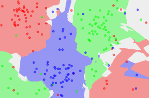
Classification can involve constructing highly non-linear boundaries between classes, as in the case of the red, green and blue classes below:
Many algorithms have been developed for automated classification, and common ones include random forests, support vector machines, Naïve Bayes classifiers, and many types of neural networks. To get a feel for how classification works, we take a simple example of a classification algorithm - k-Nearest Neighbours (kNN) - and build it from scratch in Python 2. You can use a mostly imperative style of coding, rather than a declarative/functional one with lambda functions and list comprehensions to keep things simple if you are starting with Python. Here, we will provide an introduction to the latter approach.
kNN classifies new instances by grouping them together with the most similar cases. Here, you will use kNN on the popular (if idealized) iris dataset, which consists of flower measurements for three species of iris flower. Our task is to predict the species labels of a set of flowers based on their flower measurements. Since you’ll be building a predictor based on a set of known correct classifications, kNN is a type of supervised machine learning (though somewhat confusingly, in kNN there is no explicit training phase; see lazy learning).
The kNN task can be broken down into writing 3 primary functions:
- Calculate the distance between any two points
- Find the nearest neighbours based on these pairwise distances
- Majority vote on a class labels based on the nearest neighbour list
The steps in the following diagram provide a high-level overview of the tasks you’ll need to accomplish in your code.
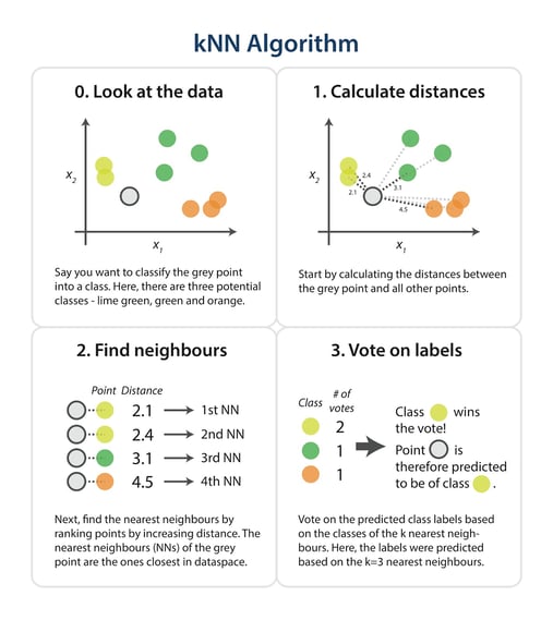
The algorithm
Briefly, you would like to build a script that, for each input that needs classification, searches through the entire training set for the k-most similar instances. The class labels of the most similar instances should then be summarised by majority voting and returned as predictions for the test cases.
The complete code is at the end of the post. Now, let’s go through the different parts separately and explain what they do.
Loading the data and splitting into train and test sets
To get up and running, you’ll use some helper functions: although we can download the iris dataourselves and use csv.reader to load it in, you can also quickly fetch the iris data straight from scikit-learn. Further, you can do a 60/40 train/test split using the train_test_split function, but you could have also randomly assigned the rows yourself (see this type of implementation here). In machine learning, the train/test split is used in order to reduce overfitting - training models on the full dataset tends to lead to the model being overfitted to the noise and peculiarities of the data, rather than the real, underlying trend. You do any sort of model tuning (e.g. picking the number of neighbours, k) on the training set only - the test set acts as a stand-alone, untouched dataset that you use to test your final model performance on.
from sklearn.datasets import load_iris from sklearn import cross_validation import numpy as np

# load dataset and partition in training and testing sets iris = load_iris() X_train, X_test, y_train, y_test = cross_validation.train_test_split(iris.data, iris.target, test_size=0.4, random_state=1)

# reformat train/test datasets for convenience train = np.array(zip(X_train,y_train)) test = np.array(zip(X_test, y_test))
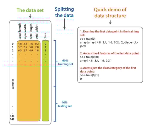
Here is an overview of the iris dataset, the data split, and a quick guide to the indexing.
Measuring distance between all cases
Given a new flower from an unknown species, you want to assign it a species based on what other flowers it is most similar to. For this, you need a measure of similarity. One such measure is the Euclidean distance, where distance d between two points (a1, a2) and (b1, b2) is given by d = sqrt((a1-b1)^2 + (a2-b2)^2)a1, a2, a3, a4) and (b1, b2, b3, b4) is simply
d = sqrt((a1-b1)^2 + (a2-b2)^2+(a3-b3)^2+(a4-b4)^2)
We’ll be making use of the zip function and list comprehensions. The zip function aggregates elements from lists (or other iterables, like strings) to return a list of tuples, such that zip([1,2,3], [4,5,6])[(1,4), (2,5), (3,6)]. List comprehensions are a powerful Pythonic construct that facilitate quick computations on lists. For example, you could quickly get the square of all numbers 1 to 100 with [pow(x, 2) for x in range(101)][x*2 for x in range(11) if x%2==1]. Here, you are iterating over values from the corresponding dimensions in the two data points, calculating the differences squared, and storing each dimension’s differences squared in diffs_squared_distance. These are then summed and returned.
import math

# 1) given two data points, calculate the euclidean distance between them def get_distance(data1, data2): points = zip(data1, data2) diffs_squared_distance = [pow(a - b, 2) for (a, b) in points] return math.sqrt(sum(diffs_squared_distance))
For example, you can now get the distance between the first two training data instances:
>>> get_distance(train[0][0], train[1][0]) 4.052159917870962

>>> get_distance(train[0][0], train[1][0]) 4.052159917870962
Or any other tuple you’d like:
<code>>>> get_distance([1,1], [2,3]) 2.23606797749979</code>
Getting the distances to all neighbours
Next, a function that returns sorted distances between a test case and all training cases is needed. One solution is the following:
from operator import itemgetter

def get_neighbours(training_set, test_instance, k): distances = [_get_tuple_distance(training_instance, test_instance) for training_instance in training_set]

 # index 1 is the calculated distance between training_instance and test_instance sorted_distances = sorted(distances, key=itemgetter(1))

 # extract only training instances sorted_training_instances = [tuple[0] for tuple in sorted_distances]

 # select first k elements return sorted_training_instances[:k]

def _get_tuple_distance(training_instance, test_instance): return (training_instance, get_distance(test_instance, training_instance[0]))
Let’s unpack these function: first, you need to calculate the distances from any given test data point to all the instances in the training sets. This can be done by iterating over each training_instance in training_set, and using the helper function _get_tuple_distance (the leading underscore indicates the function is intended for internal use only) to calculate the distance between it and the test instance. It also handily returns the training instance it’s working on (the usefulness of this will become apparent later). To test this function, try:
>>> _get_tuple_distance(train[0], test[0][0])

(array([array([ 4.8, 3.4, 1.6, 0.2]), 0], dtype=object), 1.2328828005937953)
This returns the train instances train[0] itself, followed by the distance (1.23) between it and the test[0] instance.
This pairwise calculation is done for every train instance and the given test instance. You can get a feel for what is happening with this command:
>>> [_get_tuple_distance(training_instance, test[0][0]) for training_instance in train[0:3]]

[(array([array([ 4.8, 3.4, 1.6, 0.2]), 0], dtype=object), 1.2328828005937953), (array([array([ 5.7, 2.5, 5. , 2. ]), 2], dtype=object), 4.465422712353221), (array([array([ 6.3, 2.7, 4.9, 1.8]), 2], dtype=object), 4.264973622427225)]
Next, the distances (e.g. like the 1.23, 4.47, 4.26 here) are sorted in order to find the k closest neighbours to the test instance. To understand how we can return the sorted distances, play with:
>>> distances = [_get_tuple_distance(training_instance, test[0][0]) for training_instance in train[0:3]] >>> sorted_distances = sorted(distances, key=itemgetter(1)) >>> [tuple[0] for tuple in sorted_distances]

[array([array([ 4.8, 3.4, 1.6, 0.2]), 0], dtype=object), array([array([ 6.3, 2.7, 4.9, 1.8]), 2], dtype=object), array([array([ 5.7, 2.5, 5. , 2. ]), 2], dtype=object)]
Which are the training instances ranked from closest to furthest from our test instance, as desired. The function takes the k parameter, which controls how many nearest neighbours are returned.
As a side note, instead of using a sort to order the distances from a test case in decreasing order, it would be computationally cheaper to find the maximum in the list of distances - specifically, the sort here has complexity n log(n) while passing through an array to find the maximum is O(n). If you were optimising our script for efficiency (rather than focusing on doing an educational demo), these types of considerations would become quite important.
Getting the neighbours to vote on the class of the test points
Finally, using the nearest neighbours you just identified, you can get a prediction for the class of the test instance by majority voting – simply tally up which class comes up the most often among the nearest neighbours.
from collections import Counter

# 3) given an array of nearest neighbours for a test case, tally up their classes to vote on test case class

def get_majority_vote(neighbours): # index 1 is the class classes = [neighbour[1] for neighbour in neighbours] count = Counter(classes) return count.most_common()[0][0]
The [neighbour[1] for neighbour in neighbours] just grabs the class of the nearest neighbours (that’s why it was good to also keep the training instance information in _get_tuple_distance instead of keeping track of the distances only).
Next up, Counter, which is a dictionary subclass, counts the number of occurrences of objects. Try out:
>>> Counter([7,7,7,6,6,9]) Counter({7: 3, 6: 2, 9: 1})

>>> Counter('bananas') Counter({'a': 3, 'n': 2, 's': 1, 'b': 1})
Then, the most_common method of Counter can be used to return tuples with the most common elements and their frequencies:
<code>>>> Counter('bananas').most_common() [('a', 3), ('n', 2), ('s', 1), ('b', 1)]</code>
In a similar way, you can grab the classes of the nearest neighbours, tally up how frequently the different class labels occur, and then find the most common label. This most common label will be the class prediction of the test instance.
Running our algorithm
That’s about it. Now, just string the data loading and these 3 primary functions together with a main method and run it. Let’s set k equal to 5, i.e. look at the 5 nearest neighbours to do the classification of new test instances. Once the predictions for classes of test cases are made, it would be useful to get a report of how good our predictions are. You can get these summary statistics from scikit’s accuracy_score and classification_score functions.
from sklearn.metrics import classification_report, accuracy_score

# setting up main executable method def main():

 # load the data and create the training and test sets # random_state = 1 is just a seed to permit reproducibility of the train/test split iris = load_iris() X_train, X_test, y_train, y_test = cross_validation.train_test_split(iris.data, iris.target, test_size=0.4, random_state=1)

 # reformat train/test datasets for convenience train = np.array(zip(X_train,y_train)) test = np.array(zip(X_test, y_test))

 # generate predictions predictions = []

 # let's arbitrarily set k equal to 5, meaning that to predict the class of new instances, k = 5

 # for each instance in the test set, get nearest neighbours and majority vote on predicted class for x in range(len(X_test)):

 print 'Classifying test instance number ' + str(x) + ":", neighbours = get_neighbours(training_set=train, test_instance=test[x][0], k=5) majority_vote = get_majority_vote(neighbours) predictions.append(majority_vote) print 'Predicted label=' + str(majority_vote) + ', Actual label=' + str(test[x][1])

 # summarize performance of the classification print 'nThe overall accuracy of the model is: ' + str(accuracy_score(y_test, predictions)) + "n" report = classification_report(y_test, predictions, target_names = iris.target_names) print 'A detailed classification report: nn' + report

if __name__ == "__main__": main()
This method just brings together the previous functions and should be relatively self-explanatory. One potentially confusing point may be the very end of the script - instead of just calling main() to run the script, it is useful to instead first check if __name__ == "__main__". This would make no difference at all if you only want to run this script as is from the command line or in an interactive shell - when reading the source code, the Python interpreter would set the special __name__ variable to "__main__" and run everything. However, say that you wanted to just import the functions to another module (another .py file) without running all of the code. Then, __name__ would be set to the other module’s name. This would let us use the kNN code without having it execute every time. So, this check allows the script to behave differently based on whether the script is run directly or being imported from somewhere else.
Refinements
In this implementation, when trying to classify new data points, we calculated the distance between each test instance and every single data point in our training set. This is inefficient, and there exist alterations to kNN which subdivide the search space in order to minimize the number of pairwise calculations (e.g. see i-d trees). Another refinement to the kNN algorithm can be made by weighting the importance of specific neighbours based on their distance from the test case. This would allow closer neighbours to have more of an impact on the class voting process, which is intuitively sensible.
A separate point to keep in mind is that, although here we arbitrarily chose k=5, we could have chosen other values (which would influence accuracy, noise sensitivity, etc.). Ideally, k would be optimized by seeing which value produces the most accurate predictions (see cross-validation).
An excellent overview of kNN can be read here. A more in depth implementation with weighting and search trees is here.
Full script
The full script follows:
from sklearn.datasets import load_iris from sklearn import cross_validation from sklearn.metrics import classification_report, accuracy_score from operator import itemgetter import numpy as np import math from collections import Counter

# 1) given two data points, calculate the euclidean distance between them def get_distance(data1, data2): points = zip(data1, data2) diffs_squared_distance = [pow(a - b, 2) for (a, b) in points] return math.sqrt(sum(diffs_squared_distance))

# 2) given a training set and a test instance, use getDistance to calculate all pairwise distances def get_neighbours(training_set, test_instance, k): distances = [_get_tuple_distance(training_instance, test_instance) for training_instance in training_set] # index 1 is the calculated distance between training_instance and test_instance sorted_distances = sorted(distances, key=itemgetter(1)) # extract only training instances sorted_training_instances = [tuple[0] for tuple in sorted_distances] # select first k elements return sorted_training_instances[:k]

def _get_tuple_distance(training_instance, test_instance): return (training_instance, get_distance(test_instance, training_instance[0]))

# 3) given an array of nearest neighbours for a test case, tally up their classes to vote on test case class def get_majority_vote(neighbours): # index 1 is the class classes = [neighbour[1] for neighbour in neighbours] count = Counter(classes) return count.most_common()[0][0]

# setting up main executable method def main():

 # load the data and create the training and test sets # random_state = 1 is just a seed to permit reproducibility of the train/test split iris = load_iris() X_train, X_test, y_train, y_test = cross_validation.train_test_split(iris.data, iris.target, test_size=0.4, random_state=1)

 # reformat train/test datasets for convenience train = np.array(zip(X_train,y_train)) test = np.array(zip(X_test, y_test))

 # generate predictions predictions = []

 # let's arbitrarily set k equal to 5, meaning that to predict the class of new instances, k = 5

 # for each instance in the test set, get nearest neighbours and majority vote on predicted class for x in range(len(X_test)):

 print 'Classifying test instance number ' + str(x) + ":", neighbours = get_neighbours(training_set=train, test_instance=test[x][0], k=5) majority_vote = get_majority_vote(neighbours) predictions.append(majority_vote) print 'Predicted label=' + str(majority_vote) + ', Actual label=' + str(test[x][1])

 # summarize performance of the classification print 'nThe overall accuracy of the model is: ' + str(accuracy_score(y_test, predictions)) + "n" report = classification_report(y_test, predictions, target_names = iris.target_names) print 'A detailed classification report: nn' + report

if __name__ == "__main__": main()
ABOUT THE AUTHOR

Natasha Latysheva
Natasha is a computational biology PhD student at the MRC Laboratory of Molecular Biology. Her research is focused on cancer genomics, statistical network analysis, and protein structure. More generally, her research interests lie in data-intensive molecular biology, machine learning (especially deep learning) and data science.
Interested in upskilling, reskilling or transitioning to a Data Science career?
Whether you're already working in the Data Science field, or you're looking to transition careers from a different background, we're here to help.
Please complete the form to the right of this text with your details to request an outline of our Applied Data Science Bootcamp. We'll then get in touch to talk through your career objectives.
Get in touch now
Please complete all of the required fields to get in touch with us.
-1.png)
Enquire now
Fill out the following form and we’ll contact you within one business day to discuss and answer any questions you have about the programme. We look forward to speaking with you.
