In this tutorial, we will consider a very simple linear regression model, which is the backbone of several time series and high dimensional models (VAR, Lasso, Adalasso, Boosting, Bagging, to name a few).

Linear regression assumes a linear relationship between the input variable (X) and a single output variable (Y). When there is a single input variable, the method is referred to as a simple linear regression.

In a simple linear regression, we can estimate the coefficients required by the model to make predictions on new data analytically. That is, the line for a simple linear regression model can be written as:

where Β0 and Β1 are the coefficients we must estimate from the training data and ∈ is an error term.

Once the coefficients are estimated, we can use this equation to predict output values for y conditional on new input examples of x. There are some well-known Python packages which you can use to do this model fitting for you, but here we will code this so you can understand the basics.

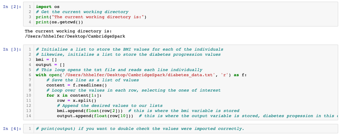
Let's begin by importing the necessary packages. We need these to plot graphs and use some simple mathematical functions such as the mean.

The diabetes dataset consists of 10 physiological variables (such as age, sex, weight, blood pressure) measure on 442 patients, and an indication of disease progression after one year. Note that the input variables have all been standardised to each have mean 0 and squared length = 1.

The dataset used here is available here

Simply save the page as 'diabetes_data.txt' to your computer desktop or ideally, to wherever your Python script is saved.

Now, we will use the below two cells to make predictions and test accuracy

We use the following formula to calculate the estimated coefficients of the line:

The quantity on the numerator is the covariance between X and Y. That is, how much they are likely to change together.

We can now show what the coefficient and intercept values are

We can confirm using the package sklearn:

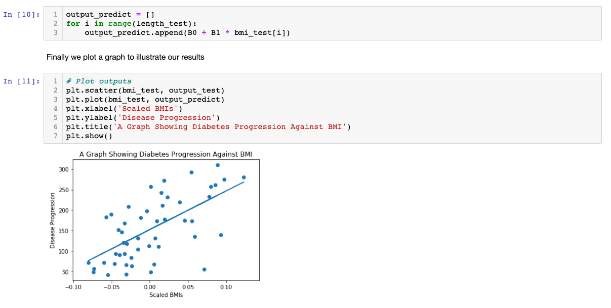
Applying the formula from the beginning of this tutorial, we can predict the diabetes progression value, based on our input variable, BMI, i.e.,

To improve this model, we could use more input variables, such as weight or blood pressure. Moreover, we can even make our own input variables from the raw data. However, one should be careful with multicolinearity issues, i.e., two or more variables are linear combinations of each other, then the parameters of the regression can't be estimated.

More Tutorials to Practice your Skills on:

– Introduction to Missing Data Imputation
– Hyperparameter tuning in XGBoost
– Introduction to CoordConv Architecture: Deep Learning
– Neural Networks in Python
– Getting started with XGBoost

By Henrique Helfer Hoeltgebaum

Henrique is currently working as a Research Associate at The Alan Turing Institute. His work includes working with Machine Learning models applied to streaming data and developing anomaly detectors to make decisions in real-time.

He attained his Master’s and PhD in Statistics from The Pontifical Catholic University of Rio de Janeiro. During his PhD he was also a visiting researcher at the Statistics department at Imperial College London. In the past he has worked as a Data Scientist and a quantitative research analyst.